Journal Article
Spatial outliers as a pattern determinant for explaining heterogeneity
https://doi.org/10.1080/13658816.2026.2682957Overview
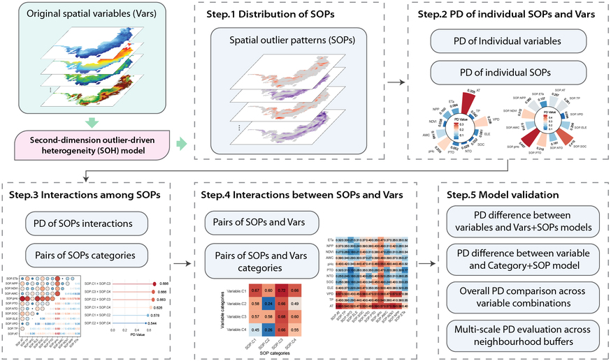
This paper introduces a second-dimension outlier-driven heterogeneity (SOH) model for explaining spatial heterogeneity with local outlier configurations. The model derives multi-scale spatial outlier patterns (SOPs), embeds them in a stratification-detection workflow, and evaluates individual, interaction, and scale-dependent effects in Australian barley production.
Abstract
Explaining spatial heterogeneity typically relies on first-dimension covariates that describe spatial gradients. However, many geographic phenomena also exhibit irregular and locally extreme structures that are difficult to capture using smooth relationships. This study proposed a second-dimension outlier-driven heterogeneity (SOH) model, in which the first dimension refers to covariate variation across space, while the second dimension represents spatial pattern information captured from local outlier configurations. SOH derives multi-scale spatial outlier patterns (SOPs) using a second-dimension outlier model and embeds them in a stratification-detection workflow, where decision tree-based stratification defines strata and the geographical detector evaluates explanatory power via the power of determinant (PD). The model supports evaluation of individual effects, SOP interactions, and SOP-variable interactions, with assessment of scale dependence across neighbourhood buffers. Application of this model to spatial heterogeneity in Australian barley production showed that SOPs strengthened heterogeneity explanation relative to original variables, and that SOP interactions and SOP-variable interactions yielded synergistic gains in PD. A scale threshold around 200 km was identified, beyond which SOP-only models approached the explanatory performance of combined models, indicating that multi-scale SOPs captured broad spatial context. Overall, SOH provides a unified approach for incorporating outlier-driven spatial patterns into spatial heterogeneity analysis.
Method Implementation
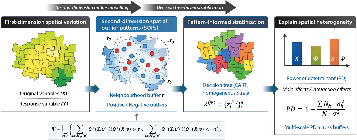
SOH explains spatial heterogeneity by adding a second dimension of spatial pattern information to conventional covariates. The first dimension is the original covariate variation across space, while the second dimension is a set of multi-scale spatial outlier patterns (SOPs) derived from local outlier configurations.
-
Prepare spatial variables on a common support
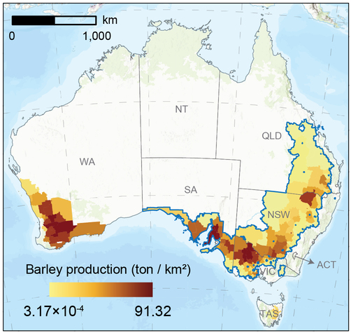
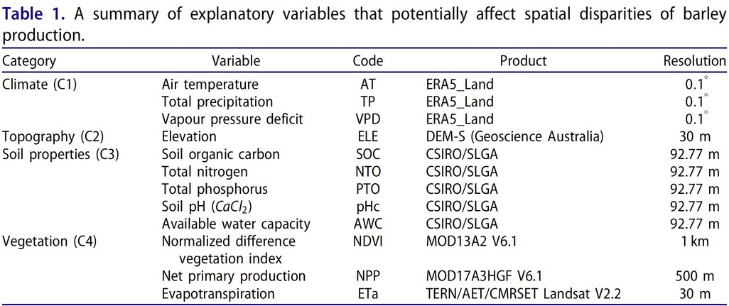
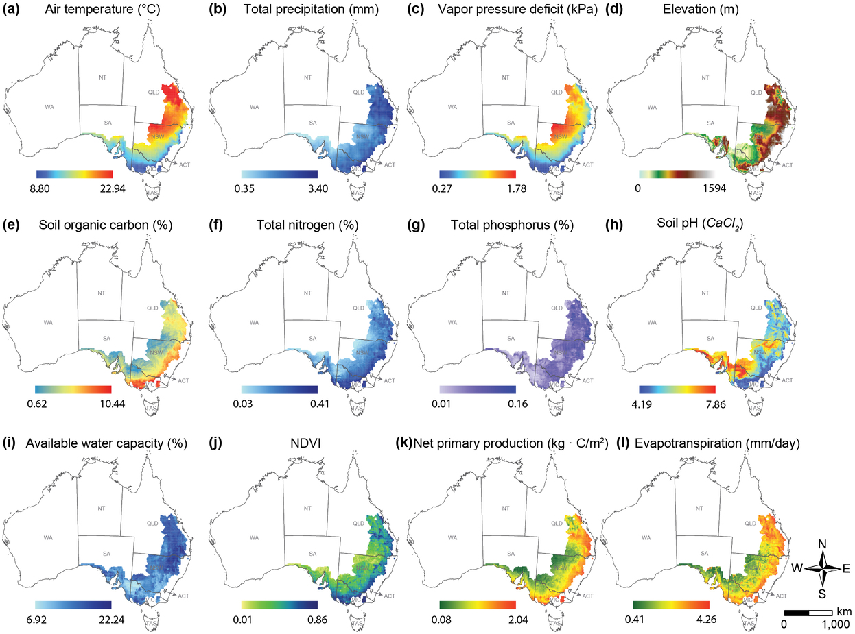
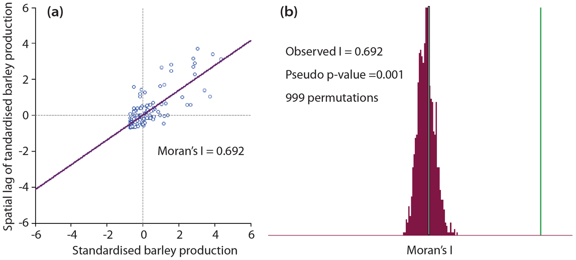
The response variable \(Y\) and explanatory variables \(X\) are first aligned on the same spatial units so that covariate values, SOPs, and heterogeneity statistics can be compared consistently. In the barley case study, the response was SA2-level barley production normalised by polygon area, and environmental predictors were harmonised to a common coordinate system and analysis grid before being aggregated to the modelling support.
-
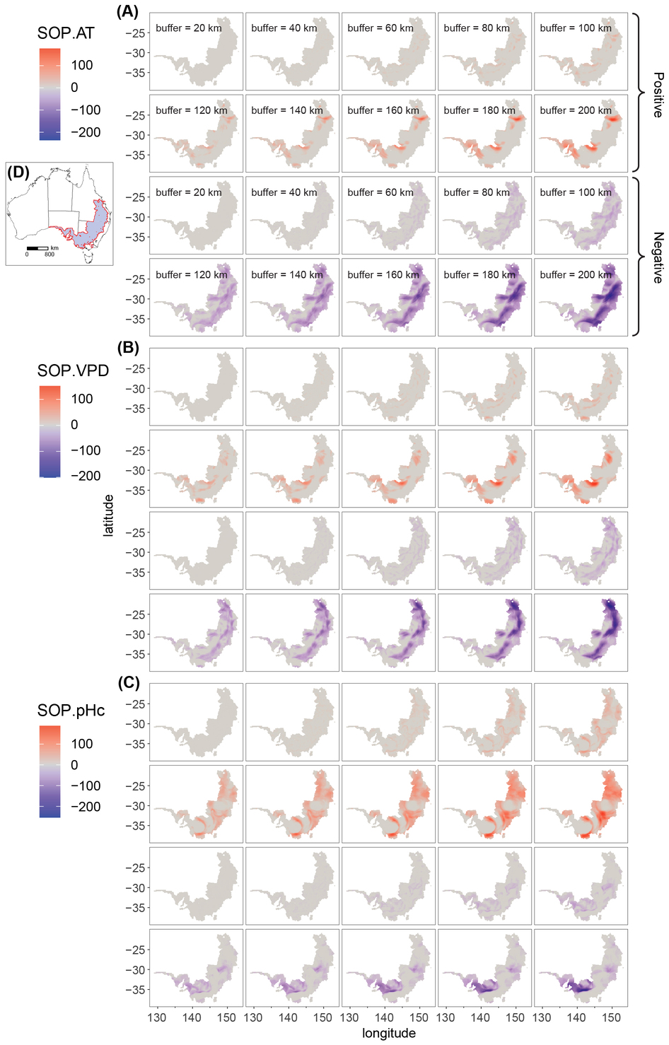
Generate multi-scale spatial outlier patterns
For each explanatory variable \(X\), SOH uses the second-dimension outlier model to identify positive and negative local deviations relative to neighbourhood distributions. Across a set of buffer radii \(R=\{r_1,r_2,\ldots,r_k\}\), the spatial pattern variable \(\Psi\) is constructed as:
\[ \Psi = \bigcup_{r \in R} \left\{ \sum_{v \in \mathcal{N}_r(u)} O^{+}(X,v)\,\mathbb{I}\!\left(O^{+}(X,v)>\tau\right), \sum_{v \in \mathcal{N}_r(u)} O^{-}(X,v)\,\mathbb{I}\!\left(O^{-}(X,v)<-\tau\right) \right\} \]Here, \(\mathcal{N}_r(u)\) is the neighbourhood around target spatial unit \(u\), \(O^{+}\) and \(O^{-}\) are positive and negative outlier components, and \(\tau\) controls the threshold for retaining pronounced local deviations. In the case study, positive and negative outliers were defined using the \(\bar{x}\pm2\sigma\) criterion, and SOPs were generated from 20 km to 200 km at 20-km intervals.
-
Build SOP variables for each spatial unit
For each spatial unit \(i\), positive and negative outlier summaries are retained at each neighbourhood scale to form the second-dimension pattern set:
\[ \Psi_i = \left\{ O^{(r_1)}_{+,i}, O^{(r_1)}_{-,i}, O^{(r_2)}_{+,i}, O^{(r_2)}_{-,i}, \ldots, O^{(r_k)}_{+,i}, O^{(r_k)}_{-,i} \right\} \]These SOP variables describe where an explanatory factor is locally enriched, depleted, or spatially unusual relative to its surrounding context. They are used as explanatory pattern descriptors rather than as residuals or noise filters.
-
Transform predictors into data-adaptive strata
SOH uses a stratification-detection strategy. A CART regression tree converts an original variable, an SOP variable, or their combination into categorical strata:
\[ Z^{(\Psi)} = \{z_i^{(\Psi)}\}_{i=1}^{n}, \qquad z_i^{(\Psi)} \in \{1,2,\ldots,L\} \]In the implementation, CART was fitted with the R package
rpartusing \(cp=0.01\), and the number of strata \(L\) was determined adaptively by the terminal nodes of the fitted tree. The tree is used here as a stratification tool, not as an out-of-sample prediction model. -
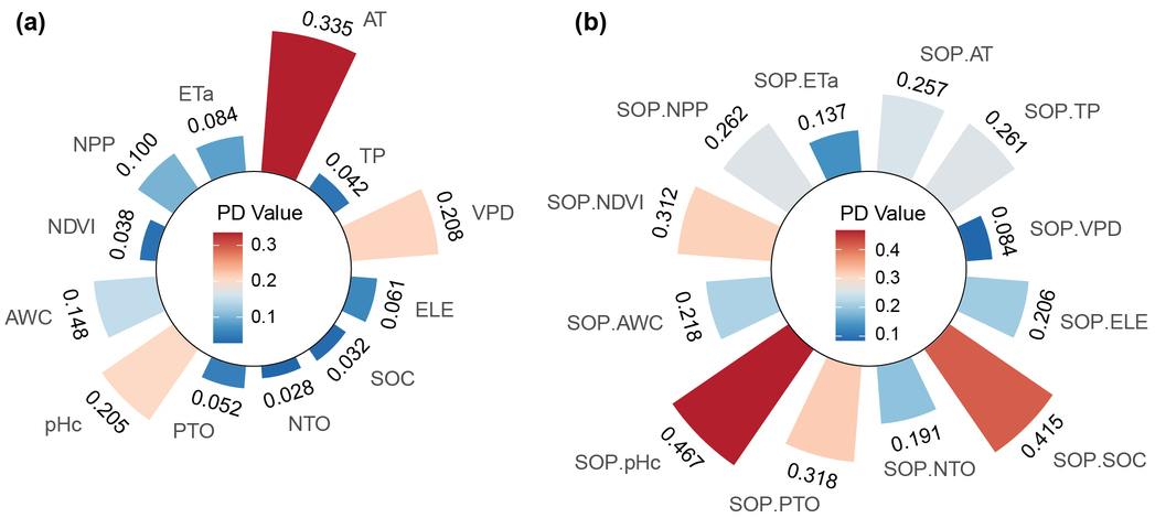
Measure explanatory power with the geographical detector
The geographical detector evaluates whether the strata induced by \(\Psi\) explain spatial heterogeneity in \(Y\). The power of determinant (PD) is:
\[ PD = \Omega_{\Psi} = 1 - \frac{ \sum_{h=1}^{L} N_h^{(\Psi)}\sigma_h^{2(\Psi)} }{ N^{(\Psi)}\sigma^{2(\Psi)} } \]A larger PD indicates that the constructed strata produce stronger between-stratum differentiation and lower within-stratum variance, meaning stronger explanatory power for spatial heterogeneity.
-
Evaluate original variables, SOPs, interactions, and scale effects
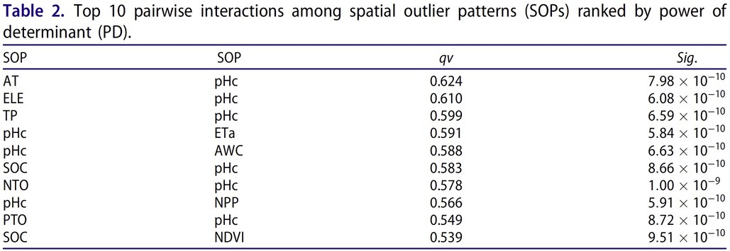
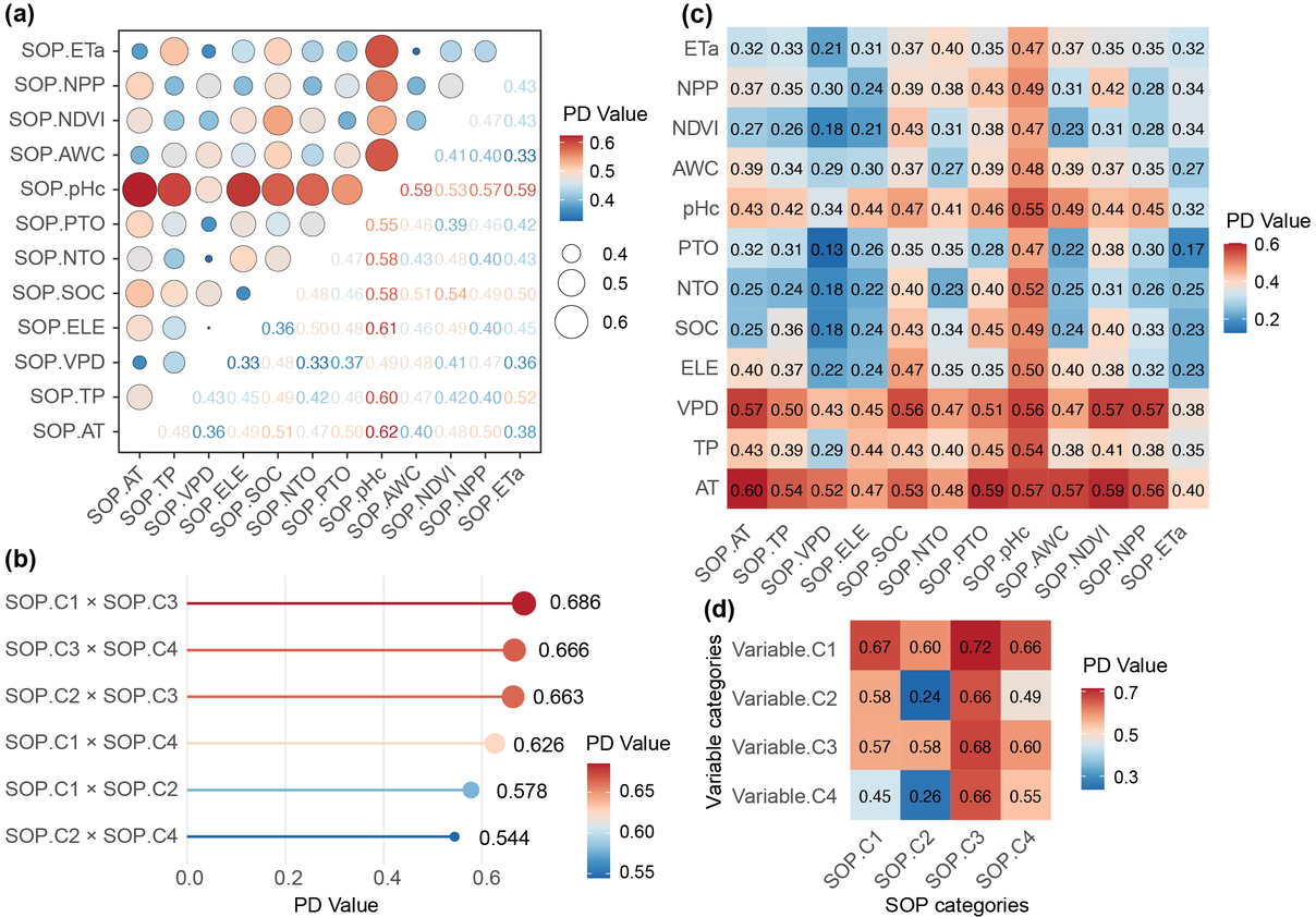
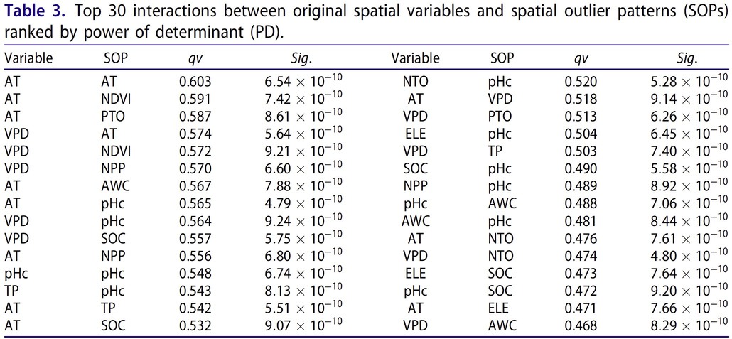
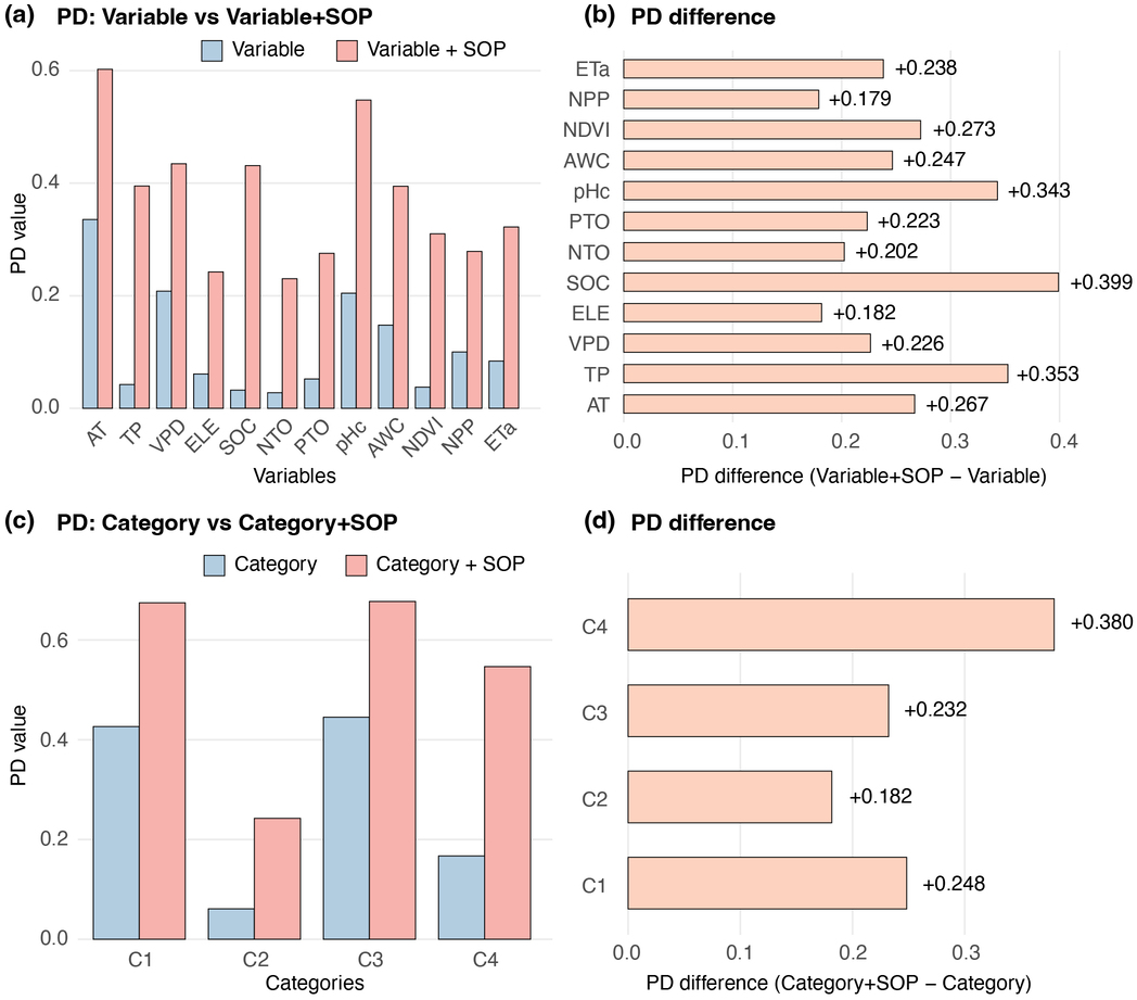
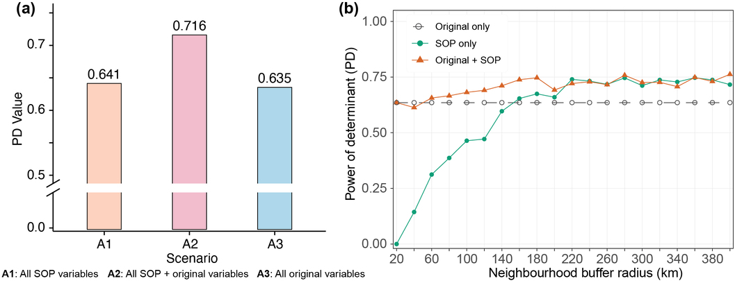
PD is calculated under several predictor configurations: original covariates \(X\), SOP variables \(\Psi\), and combined sets \(X \cup \Psi\). The same framework is then used to test pairwise SOP interactions, interactions between SOPs and original variables, category-level interactions, and the sensitivity of PD to neighbourhood buffer size. In the paper, this workflow showed that SOPs added explanatory power beyond original variables and that the SOH response stabilised around a neighbourhood threshold of approximately 200 km.
Figures and Tables
Data and Code Availability
The data and code supporting this study are publicly available through both Figshare and GitHub.
Funding
This research was supported by the National Natural Science Foundation of China (Outstanding Young Scholars Program, Grant No. 42325107).