Journal Article
Second-dimension outliers for spatial prediction
https://doi.org/10.1080/13658816.2025.2580414Overview
This paper introduces second-dimension outliers (SDO) as a new way to encode the outlier context around unsampled locations and then uses SDO-enhanced machine learning to improve spatial prediction of wheat production across Australia.
Abstract
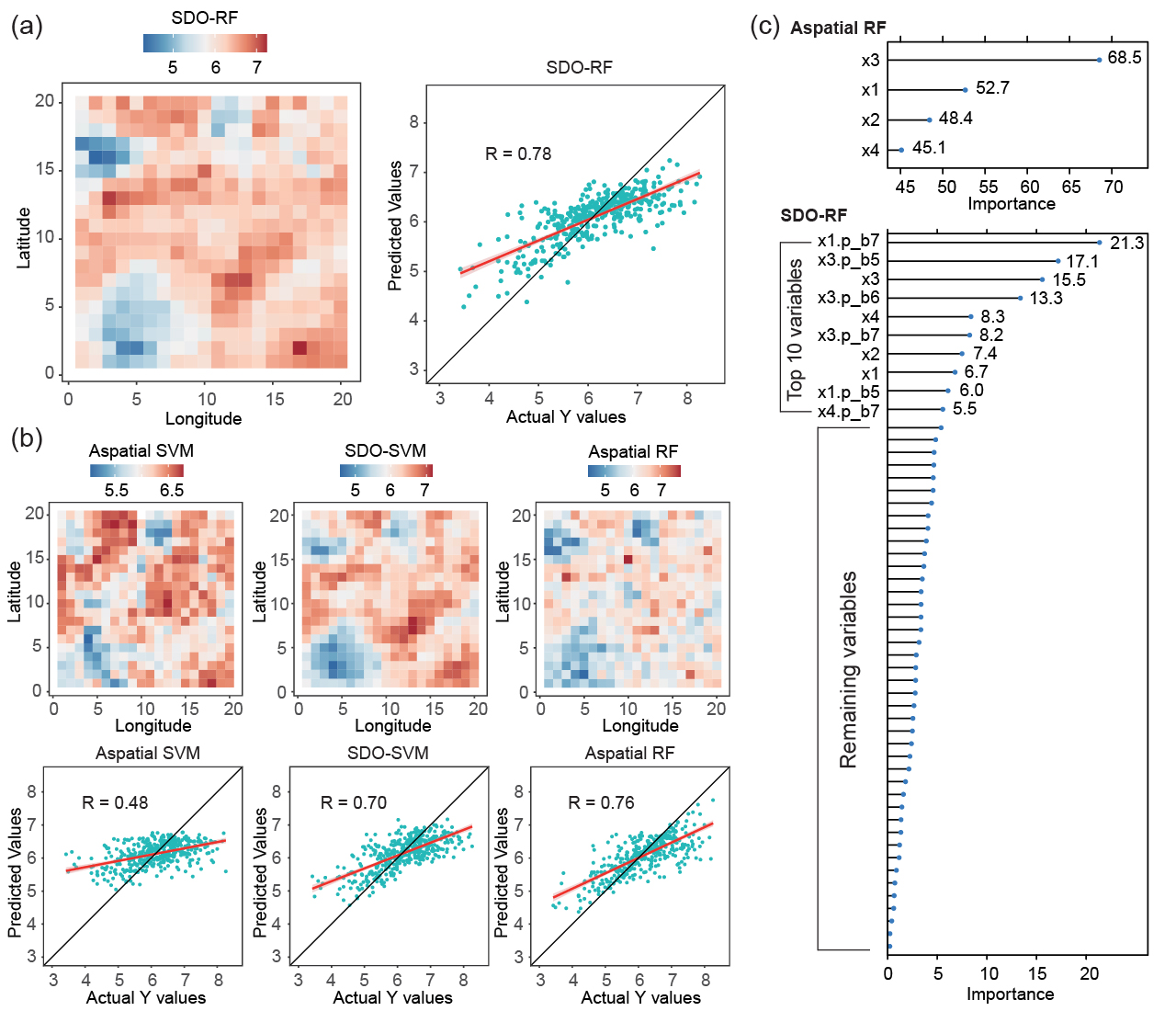
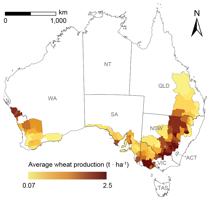
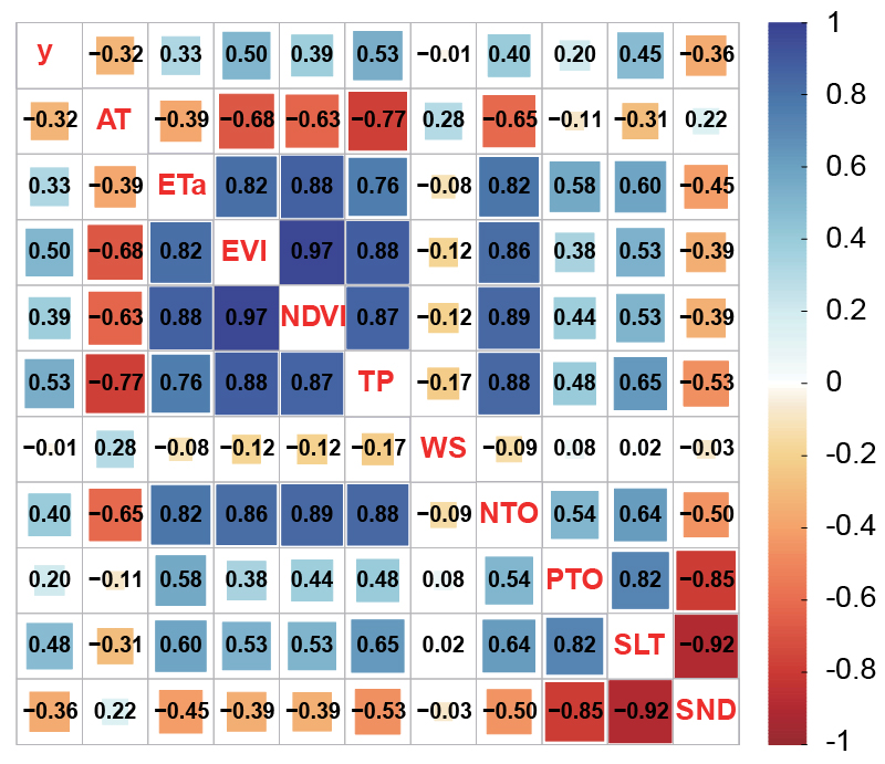
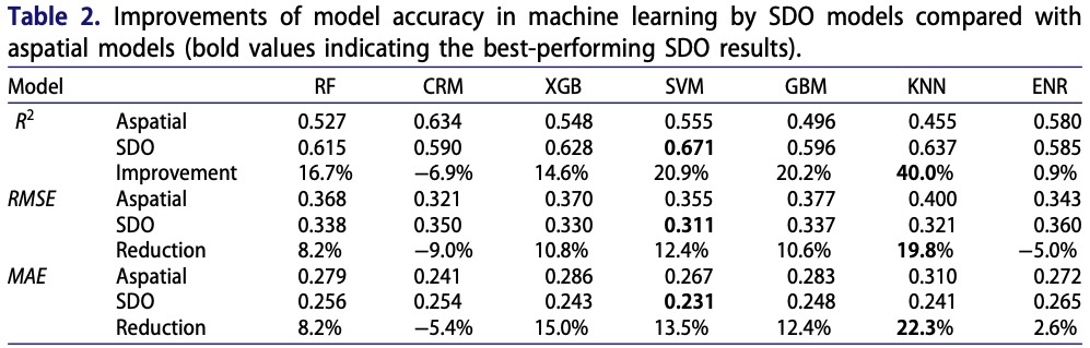
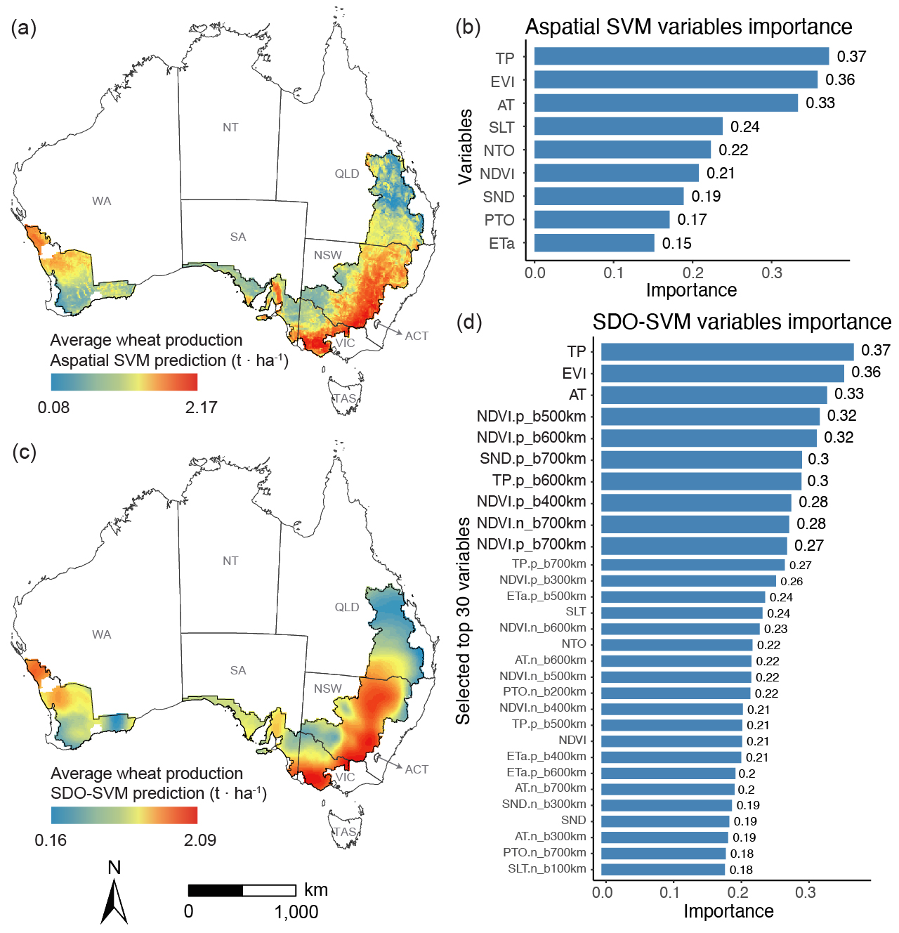
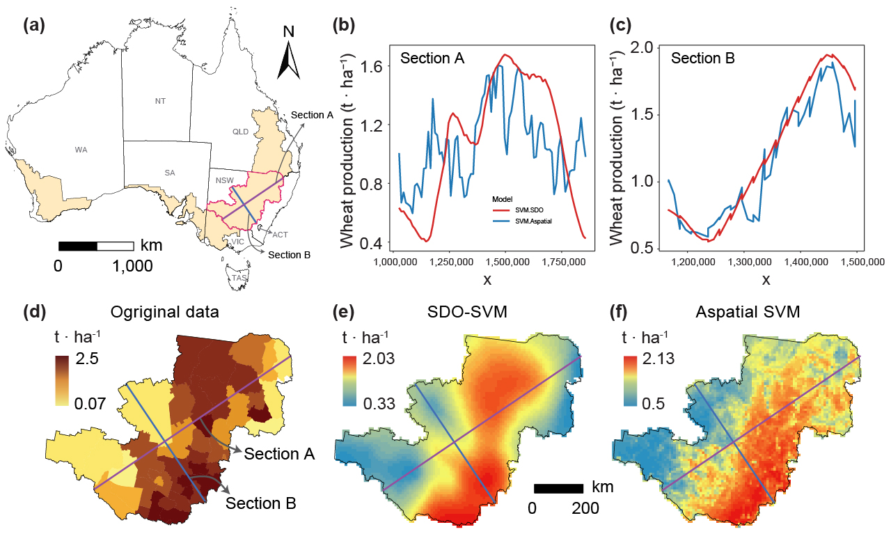
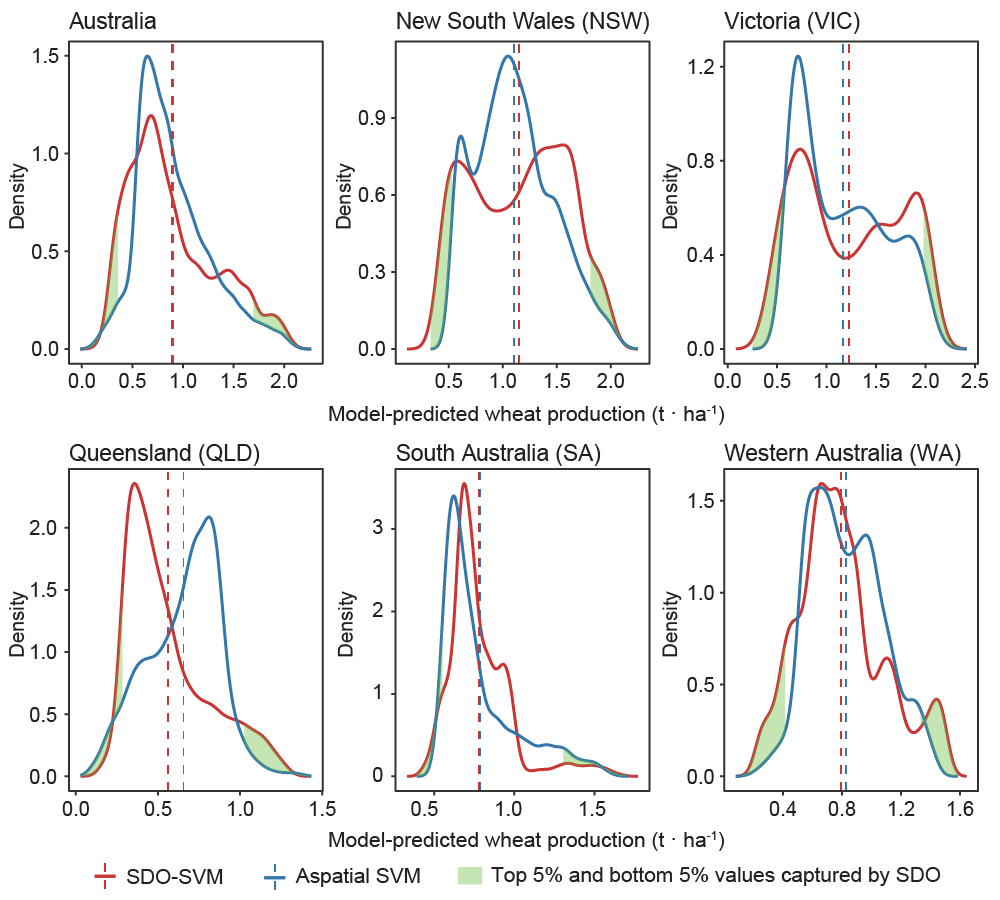
Spatial prediction aims to accurately estimate attributes at unsampled locations based on spatial dependencies, patterns, variability, and covariates, providing knowledge of complex spatial systems and supporting diverse applications. However, existing methods for spatial prediction ignore geographic and environmental characteristics outside sample locations, particularly spatial outliers, significantly impacting prediction accuracy. This study introduces the concept of second-dimension outliers (SDO) and SDO models that incorporate local outlier information at unsampled locations to enhance prediction accuracy. SDO models generate SDO variables that capture samples' external geographic and environmental characteristics in the spatial prediction. This study develops SDO-based machine learning to predict wheat production in Australia, using cross-validation to evaluate prediction accuracy. Results demonstrate that SDO-based support vector machines (SVM) improve spatial prediction accuracy, with the R2 increasing from 0.555 to 0.671 compared to aspatial SVM, particularly for extreme values. The developed local outlier strength index that examines the strength of SDO ensures more accurate and smooth spatial predictions. The SDO concept provides more in-depth explanatory information from an innovative spatial perspective and a detailed understanding of local outliers for spatial prediction, making it a robust and effective tool for spatial statistical inference and geographic computation across various fields.
Method Implementation
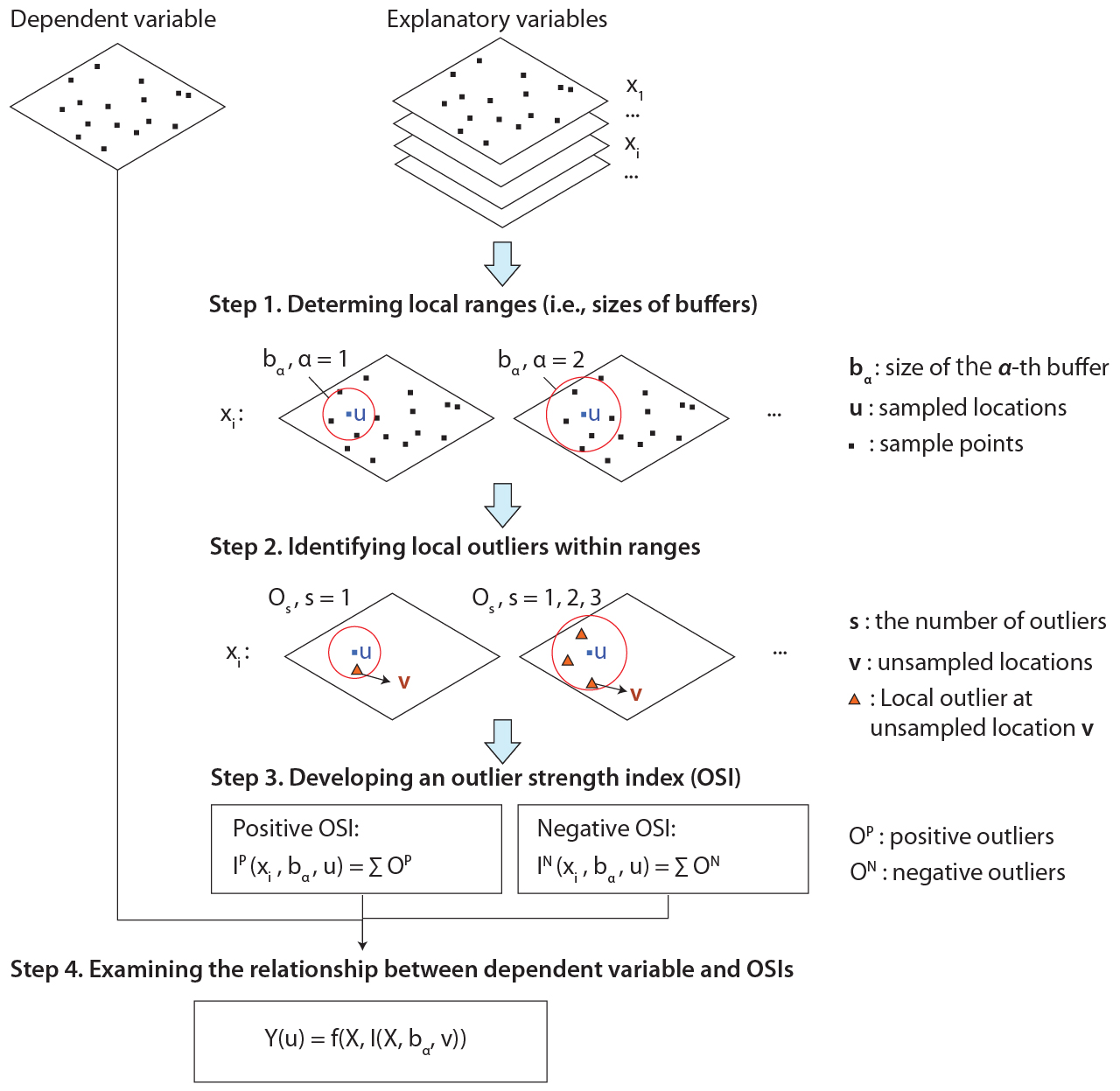
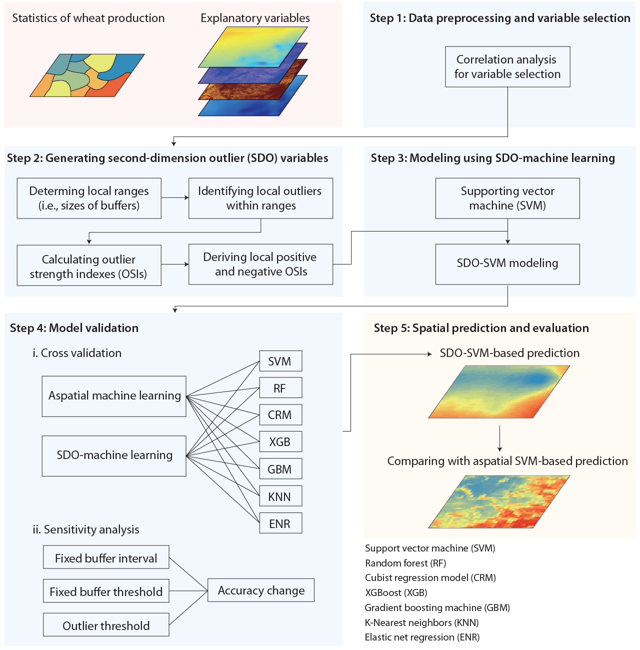
The SDO model improves spatial prediction by extracting local outlier information from explanatory variables around sampled locations and converting that information into second-dimension variables. These variables are then combined with the original covariates in machine-learning models, so outliers are not removed; their local strength is quantified and used as additional spatial context.
-
Define sampled and unsampled spatial supports
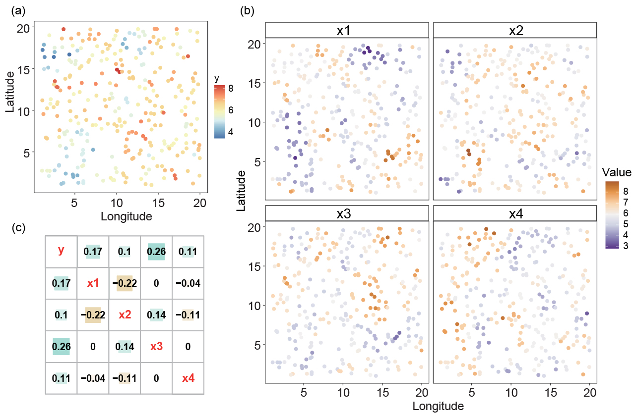
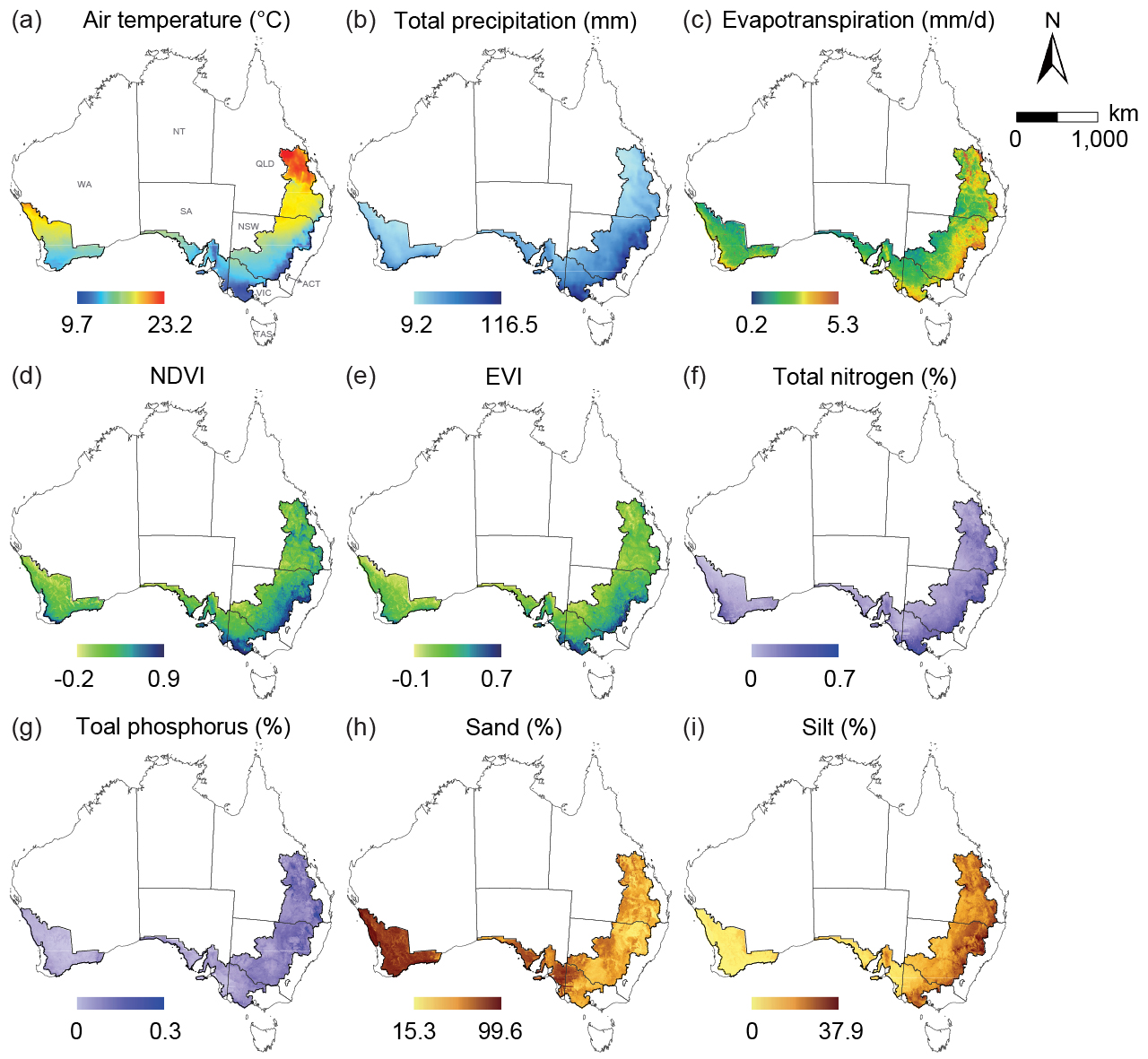
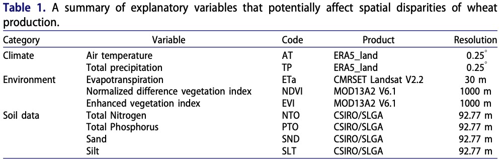
Let \(u\) denote sampled locations where the dependent variable is observed, and let \(v\) denote unsampled grid locations or surrounding locations outside the dependent-variable samples. The original covariates \(X\) are available over the prediction domain, allowing local outlier information around each sampled location to be extracted from nearby unsampled locations.
-
Select local buffer ranges
A set of local ranges is defined around each sample point so that outlier information can be measured at multiple spatial scales:
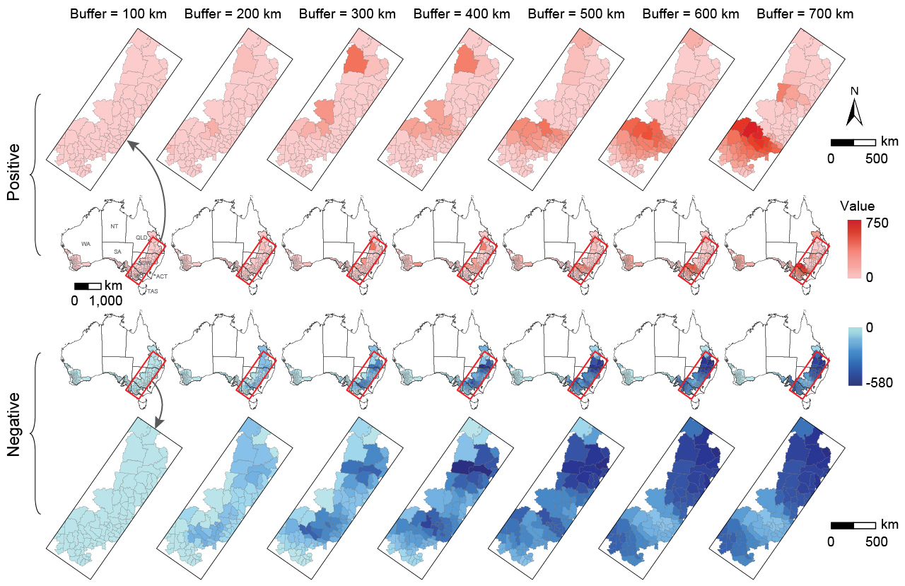
\[ b_\alpha,\qquad \alpha = 1,2,\ldots,m \]In the simulation experiment, six buffers from 2 to 7 were used. In the wheat production case study, seven buffer distances from 100 km to 700 km at 100-km intervals were used, balancing spatial context, computational efficiency, and statistical reliability.
-
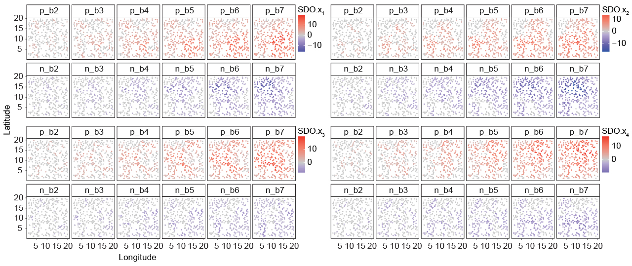
Identify positive and negative local outliers
Within each buffer, values at surrounding locations are compared with the local distribution. Positive outliers exceed \(\bar{x}+2\sigma\), while negative outliers fall below \(\bar{x}-2\sigma\). For an explanatory variable, the local outlier vector around location \(u\) is:
\[ O_s(u),\qquad s=1,2,\ldots,n \]Here, \(O_s(u)\) represents outlier values at unsampled locations \(v\) within the buffer around \(u\), and \(n\) is the number of detected outliers in that buffer.
-
Compute outlier strength indices
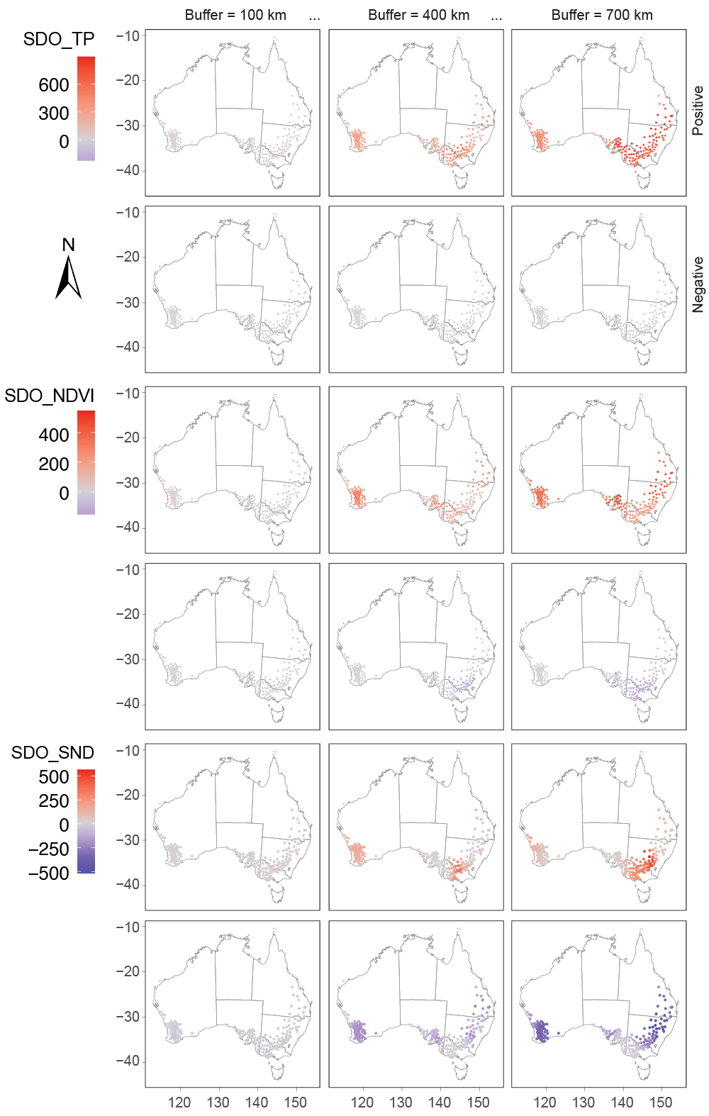
The outlier strength index (OSI) summarises the cumulative magnitude of positive and negative outliers for each explanatory variable and buffer distance:
\[ \begin{aligned} I^P(X,b_\alpha,v) &= \sum_{s=1}^{m} O^P_s(b_\alpha,v),\\ I^N(X,b_\alpha,v) &= \sum_{t=1}^{n} O^N_t(b_\alpha,v),\\ I(X,b_\alpha,v) &= \left[ I^P(X,b_\alpha,v), I^N(X,b_\alpha,v) \right] \end{aligned} \]Each buffer produces one positive and one negative SDO variable for each explanatory variable. In the wheat case, this generated 14 SDO variables per original predictor across the seven buffer distances.
-
Train SDO-enhanced machine-learning models
The original covariates and their SDO variables are combined as the model input:
\[ Y(u) = f\!\left( X,\, I(X,b_\alpha,v) \right) \]The function \(f(\cdot)\) can be implemented with machine-learning algorithms such as RF or SVM. In the real-data application, the best-performing model was SDO-SVM with a Gaussian radial basis function kernel:
\[ K(\vec{x_i},\vec{y_i}) = e^{-\gamma\left\|\vec{x_i}-\vec{y_i}\right\|^2} \] -
Validate prediction accuracy and robustness
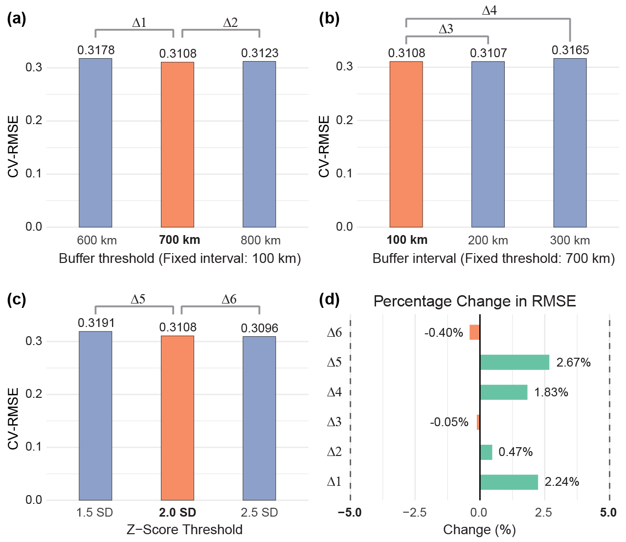
The SDO-enhanced models are compared with their aspatial counterparts using five-fold cross-validation and metrics including \(R^2\), RMSE, and MAE. The case study compared SDO-SVM, SDO-RF, SDO-CRM, SDO-XGB, SDO-GBM, SDO-KNN, and SDO-ENR against corresponding aspatial models. Sensitivity analysis then tested buffer threshold, buffer interval, and outlier threshold settings; the preferred case configuration used a 700 km buffer threshold, 100 km interval, and \(\bar{x}\pm2\sigma\) outlier criterion.
Figures and Tables
Data and Codes Availability Statement
The data and codes that support the findings of this study are available through both Figshare and GitHub.
Funding
This research was supported by the China Scholarship Council (Grant No. 202206300058).